Instruction level parallelism: An introduction to computer architecture

This page was made to support and compliment a presentation with these slides.

Purpose

• Convince you that software developers should care about architecture
• Show you how to exploring how code runs on hardware
  • Highly advanced technology. In physics or chemistry, the most advanced technology is very expensive, only available in hard to access certain labs. In computer architecture, the most advanced technology is on your laptops, and in open source software.
• Show you some really fun stuff

Parallelism

Basic circuits are inherently sequential: one transistors needs to switch before the next one can, and that switch is a physical change that takes time.

You can make the transistors change faster by increasing voltages. Unfortunately, using this technique there is a rather unfortunate physical property where \(\text{Power} = \text{Clock speed}^2\), so quite quickly, your silicon chip will simply melt if you increase the voltage to increase clock speed.

What this means in practice is that there is a limit to how much you can increase speed by increasing voltage. In fact, that point was reached a long time ago.

Meanwhile, More’s law continues:

So how can we use those extra transistors?

Here is an idea: instead of trying to use 1 circuit faster, lets try to use a bunch of circuits at the same time. In other words, lets try running our computations in parallel.

What is parallelism?

Before running a computation, you often need other computations to be run first.

From a hardware perspective, you can view this as circuit depth. From a software perspective, you can see this as data dependency chain.

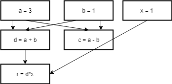
Here is some silly example code

a = 3
b = 1
d = a + b
c = a - b
x = 1
r = d * x

Here is a dependency graph of the code

You can also do this for arbitrarily long code. The idea of “reductions” (as in the MapReduce paradigm) is based on this.

sum = 0
sum += a[0]
sum += a[1]
sum += a[2]
sum += a[3]

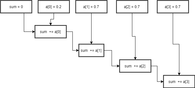
This has a circuit depth of 4. How can you lower that depth?

Well, addition is associative, so what if we start adding the middle?

sum1 = 0
sum1 += a[0]
sum1 += a[1]
sum1 += a[2]
sum2 = 0
sum2 += a[3]
sum2 += a[4]
sum = sum1 + sum2

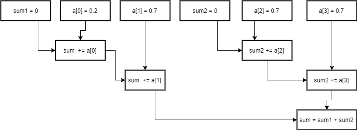
This has a depth of 3, so we made it faster. You can generalize this process to n associative operations, resulting in depth of log(n).

Hopefully you can believe that this is a general and powerful method of identifying parallelism. In fact, we are very close to an nice theory of optimal parallelism.

The famous complexity textbook Introduction to the Theory of Computation by Michael Sipser uses the following definition of parallel complexity.

Parrelell time complexity of a boolean circuit is its depth, or the longest distance from an input variable to the output gates

All sorts of nice things arise out of this definition. You can define optimal speedup with a parallel processor to be:

Which is easy to analyses with napkin based calculations.

You can also get some nice theoretical results out of this (Sipser focuses on this).

So I think we are on to something really core to what we mean by parallelism.

So now that we know what to look for when trying to parallelize things, lets go back to the hardware.

Brief introduction to assembly

Hardware is essentially an interpreter. Conceptually, it reads the code 1 line at a time, and processes it, and moves on to the next line.

So, as you might expect, the way computers look at code is as a sequence of commands. The syntax reflects this concept.

As I also want some real world examples, I will introduce you to the basics surrounding x86 assembly, which is ubiquitous in desktop and laptop CPUs. Not of any fondness of the language (it is unnecessarily complex), but because you can actually execute it on your machine.

I do have a warning: x86 is complicated, and there aren’t good tutorials like there are with C. You won’t be able to learn everything without much months of effort. Hopefully I can convince you to try to reason about assembly at a higher level, and not really worry about the details for now (your compiler can take care of that). So when reading the next couple sections, try to take it lightly, and get a feel for how it looks.

x86 in GAS (GNU Assembly syntax) looks more or less like the following:

<command> <src> <dest>

There are a set of common commands you will always see:

add/sub/mul:    basic arithmetic
lea:            pointer arithmetic
sar/sal:        bit shifting (pos/neg powers of two)
cmp/test:       ordinary and logical and based comparison.
je/jne/jle <LOCATION>:  If the comparison is equal/not equal/less than or
            equal, "jump" to LOCATION (next instruction will be executed there)

The src and dest can either be registers, or references to memory specified by registers. You can think of registers as a hardware form of local variables.

`%rax` is a register.
`(%rax)` is a reference to a memory location specified by `%rax`. This is equivalent to `*(ptr)` in C.  
`4(%rax)` is an offset of 4 bytes from the pointer, equivalent to `*(4+char_ptr)` in C.

Floating point arithmetic is a little different. The registers are called xmm0 for 128 bit registers, and ymm0 for 256 bit registers (yes, the first 128 bits of ymm0 are exactly xmm0). The idea is that each float in them is only 32 or 64 bits, but there can be several in a single register. You can also do computations on lots of integers in them, but that is less common.

Basic command format is

<cmd><p/s packed/single><s/d single/double>

Packed means you move the whole vector, single means you move the first element.

The float type in C is 32 bits, the double type is 64 bits.

Some examples

movps 16(%rcx), %xmm0   //move packed (128 bits of) data starting from 16 bytes off %rcx to %xmm0
addss %xmm0, %xmm1      //add first single precision float (32 bits) of %xmm0 to first one in %xmm1
movss %xmm0, 16(%rcx)   //move first 32 bits of %xmm0 to 16 byes off %rcx

There is also some archaic floating point arithmetic which is horribly slow, but it can work on 80 bit floats. If you ever see anything like fld or fadd, then you can check it out here.

There is a lot of other things you can learn, which may be important. There are integer vector instructions as well. And vector instructions are not the only important ones: mulx is a recently added instruction for cryptography, and it operates on regular registers.

References

You can do almost everything you can with assembly with compiler intrinsics (decent overview on microsoft’s site).

Here is an amazing reference on intel’s intrinsics. I have learned more about x86 from this site than from any assembly reference: https://software.intel.com/sites/landingpage/IntrinsicsGuide/. This is implemented on gcc, clang, vcc, and icc.

On the other hand, if you really do want to write x86 assembly, then you will need good references. Here are some of the more complete ones.

Oracle docs. Fairly well organized. https://docs.oracle.com/cd/E18752_01/html/817-5477/ennbz.html

Scraped from official docs: http://www.felixcloutier.com/x86/

Official intel docs, many pdf volumes: https://software.intel.com/en-us/articles/intel-sdm

x86 Example

How do you get assembly? You can write it yourself, of course. But people rarely feel the need to these days, because the compiler generates it for them. However, c and c++ programmers often look at what their compiler is generating. After all, sometimes the compiler isn’t perfect, and so it is nice to see what it is actually generating, in case you think it might be screwing up.

To get gcc to generate assembly, you call

gcc -S <file>

You can also plug in your code at this cool website which outputs assembly. This is especially cool as you get to see the difference in output between several different compilers.

Here is some very simple c++ code that multiplies a scalar by a vector of doubles.

#include <vector>
using namespace std;

void vector_scalar_mul(vector<double> & vec, double scalar){
    int vec_size = vec.size();
    for(int x = 0; x < vec_size; x++){
        vec[x] *= scalar;
    }
}

Here is the generated assembly.

.LFB780:
	movq	(%rcx), %rax 	//rax = argument(1)
	movq	8(%rcx), %rdx	//rdx =
	subq	%rax, %rdx		//
	sarq	$3, %rdx
	testl	%edx, %edx
	jle	.L5
	subl	$1, %edx
	leaq	8(%rax,%rdx,8), %rdx
.L4: // Main loop of vector_scalar_mul function
	movsd	(%rax), %xmm0	//
	addq	$8, %rax
	mulsd	%xmm1, %xmm0
	movsd	%xmm0, -8(%rax)
	cmpq	%rdx, %rax
	jne	.L4
.L5:
	ret

Lets go through this quickly. Because we are only concerned about performance, we can ignore large parts of it.

This is mostly crap that deals with how functions are called. The first few commands of any function will probably involve stuff like this, moving things to or from memory, and subtracting pointers.

movq	(%rcx), %rax 	//load argument 1
movq	8(%rcx), %rdx	//load argument 2

A early exit condition. Basically, this is a trick to get it to exit faster if the function isn’t actually doing any work. It can also can make the inner loop faster. You can usually spot these things because they always involves some conditional branch, and often lots of shifting and subtraction.

subq	%rax, %rdx		//???
sarq	$3, %rdx   //rdx /= 8
testl	%edx, %edx //%edx == 0
jle	.L5            //if the above condition is true, return

Setting up the pointers in the inner loop so that there is less arithmetic that needs to happen to access arrays. This is fairly critical in fast code, there is some reason for concern if you don’t see something similar to this before your loops. You can spot this from the lea command, and also that it is operating on pointers that are changed in the main loop.

subl	$1, %edx
leaq	8(%rax,%rdx,8), %rdx

One thing to note is that all of the above code can run crazily fast. It will usually not make a noticeable difference in code performance.

This next part is the important part, and the part that can be slow: our inner loop.

.L4:
	movsd	(%rax), %xmm0   
	addq	$8, %rax
	mulsd	%xmm1, %xmm0
	movsd	%xmm0, -8(%rax)
	cmpq	%rdx, %rax
	jne	.L4

Why is this slower? Well, because it is run on each element of the vector. So this runs in O(n) time, while the rest of the function runs in O(1) time. Also, floating point multiplication operation mulsd has a higher latency than other instructions, i.e., it take 3 cycles to complete, where addq, cmpq only take a single cycle. This turns out to not be very important here, but in other cases, it can be critical.

Timing code

How many clock cycles does this inner loop actually take? Timing the time it takes to run one has a great deal of variance, so lets just run it a bunch of times, and average.

So I wrote a fairly simple loop code that runs the vector_scalar_mul function a bunch of times. Then, we can easily see exactly how fast the function runs by simply looking at the time spent running the code.

g++ -O2 pipelined_floats_exec.cpp
time ./a.exe

    real    0m0.477s    # (this is the one we usually care about)
    user    0m0.000s
    sys     0m0.015s

My loop runs the function 1,000,000 times on vectors of length 1000. this means the inner loop is running about 2 billion times per second.

Since my machine usually runs at roughly 3ghz, this means the inner loop takes at most 3/2 of a clock cycle. How it is possible to run 5 instructions, including one that takes 3 cycles to complete, in less than 3/2 of a cycle?

It turns out that amazingly enough, the hardware analyzes the sequential instructions and builds data dependency graphs to see which instructions can be run in parallel, and then runs them in parallel.

But this is highly non-trivial, and is worth exploring in more detail.

Instruction level parallelism

In a conceptual perspective, when designing circuits and software, there is only kind of one dependency: data dependencies (as talked about in the beginning).

But when making programmable machines in the Von Neumann architecture, there are a lot more dependencies and everything becomes much more complicated.

Lets look at an example of some code, and the dependencies it has.

Ideal model of data dependencies

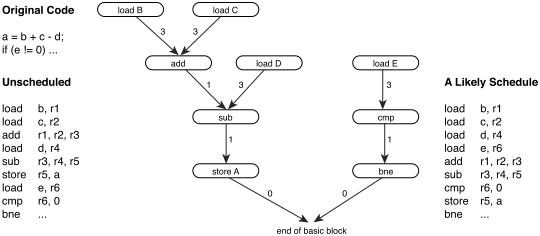
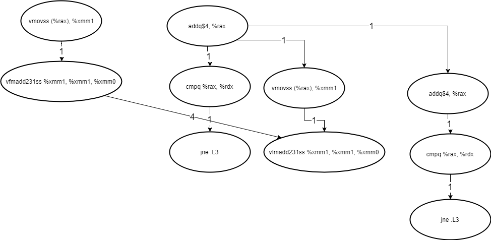
Instruction dependencies

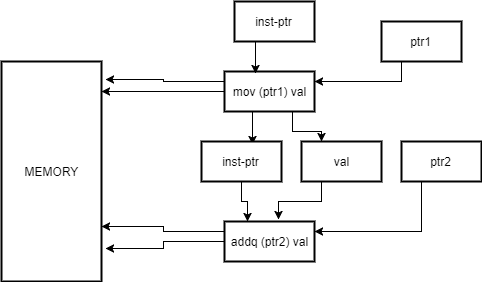
Machine code is simply 0s and 1s in memory. There are pointers to the current instruction, and code is fetched rather similarly to data. The problem is, that like data, each instruction can change the pointer to the next instruction arbitrarily. Function calls and branches do this. The worse case is a call to a function pointer, which cannot be determined before the pointer is calculated, so there is really no hope of ever completely fixing this dependency.

But even in simple examples, it is tricky. In a really naïve implementation, we cannot remove the circled dependence below because we simply do not know if the instruction will change that pointer until we have already loaded and executed it.

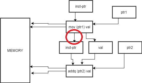
But luckily for us, modern hardware is not naive, and contains lots of sophisticated techniques to handling this problem.

The main one is called branch prediction, and we can get to that later.

Memory dependencies

These are the closest to data dependencies. We simply need to be able to access data that we have stored at some point.

Unfortunately, accessing data is really, really slow. These days, a single access to data on global RAM usually takes around 100 clock cycles. We are getting data all the time, so really, we could be spending ~99% of the time just fetching data.

And that is only the start of the massive performance problems with memory. The details are out of the scope of this paper, but I think it is a really fun and cool field that is at least as important as parallelism and dependency analysis. Ulrich Drepper wrote a free online book describing in detail everything you could ever want to know about memory https://www.akkadia.org/drepper/cpumemory.pdf.

Circuit dependencies

Conceptually, we can just add more circuits onto a piece of paper. However, in reality hardware has a fixed number of circuits, each can only be calculating one value at a time.

Pipelining

Superscalar dispatch

Compiler optimizations

One easy way people try to make things faster is enable compiler optimizations. The idea is that the compiler puts aditional transformations on your code to make it run faster. This allows the software to effectively exploit many of the hardware features we have discussed.

Here is how to turn on optimizations for the vector_scalar_mul function.

g++ -O3 -march=haswell pipelined_floats_exec.cpp
time ./a.exe

    real    0m0.169s
    user    0m0.000s
    sys     0m0.015s

Recall that with -O2 level of optimization, we got 0.477s. So it got nearly 3 times faster.

For most purposes, people just treat assembly generation as a black box. You simply give gcc the -O2 or -O3 option, and trust that it makes your code faster. Unfortunately, for our purposes, we cannot treat the compiler optimizations as a black box. Modern compilers really are amazing, but they are not yet perfect. Understanding how to guess, observe, and measure the level to which they are not perfect is key to understanding how your code executes on hardware.

How your compiler sees code

To understand our compiler, we need to get inside its head. How does it see code, how does it work with it?

function addA(d) {
    var a = 42;
    return a + d;
}
var c = addA(2) + 3;

Here is a basic parse tree of the code, generated at this cool page.

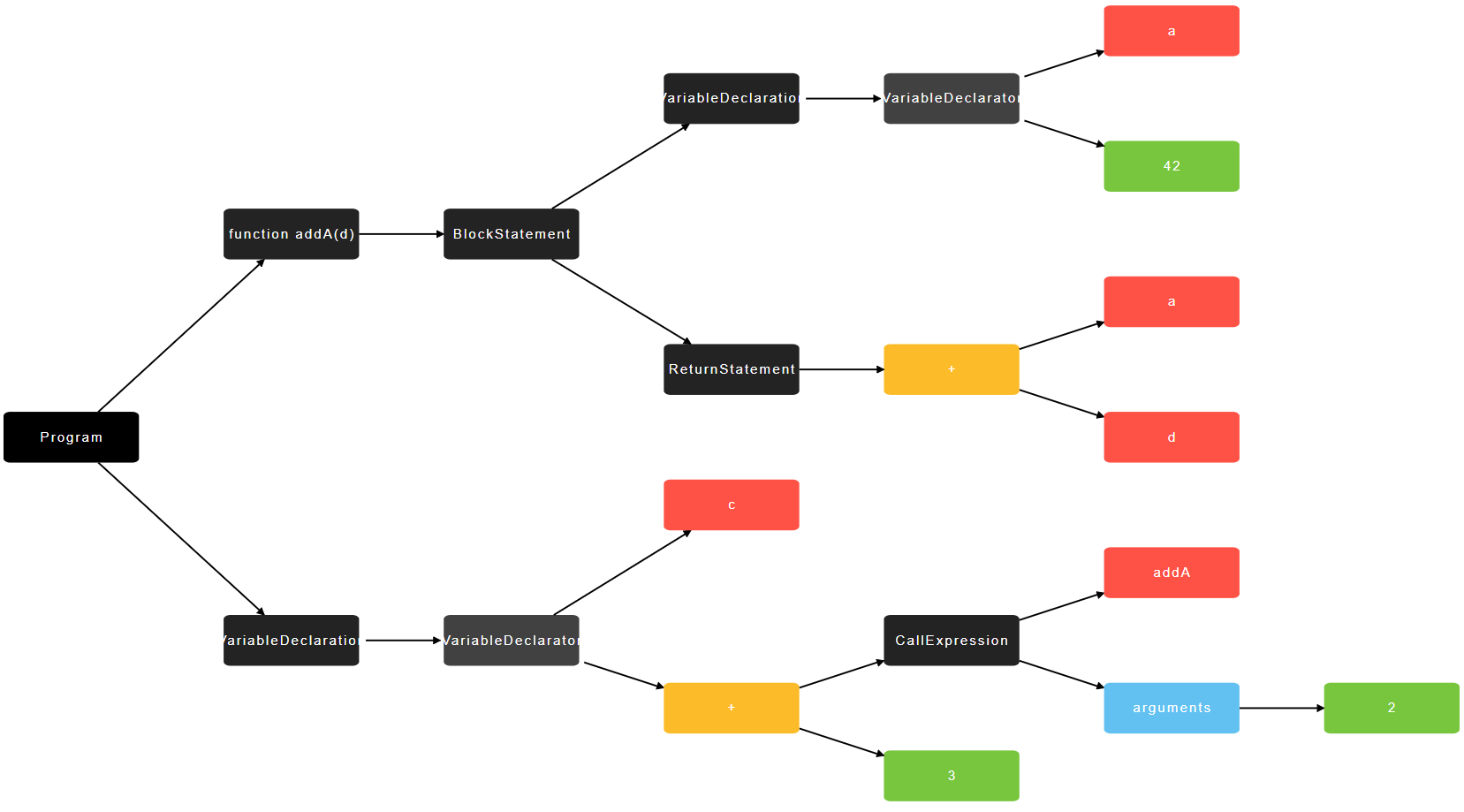
This is the first representation of code, the parse tree.

Note that the details of how things are parsed changes from compiler to compiler. But the idea is the same. Expressions are nodes of

Then you go into the intermediate representation. This can be very simple (10 kinds of statements in Haskell Intermediate language), or very complex (hundreds of operators and annotations in LLVM IR).

Static dependency analysis

Simple static assignment

More resources:

Instruction scheduling

Types of parallelism

• “Invisible” Parallelism
  • Instruction pipeline
  • Superscalar dispatch
  • Vector instructions
• Visible parallelism
  • Multi-core CPUs (threads)
  • GPGPUs?

I will go through these one by one, explaining how they work.

“Invisible” Parallelism

When computer architects started realizing they had more transistors than they could use in sequential instruction, they knew that the code would have to be run in some kind of parallel manner.

They also knew that software developers are lazy and don’t want to change their code.

The solution is to take code which the software developer thought was completely sequential, but actually execute some of it in parallel.

The following will be a touch on some of the techniques the computer architects and compilers came up with to run sequential code in parallel.

Assembly

To explain the concepts fully, I have to bring in assembly code. However, I will translate the x86 back into a c like psedo-assembly, that is hopefully more accessible.

Code dependency graphs

In code, there are obvious dependencies on previous code executing. For example,

    a += b
    a *= c

Clearly, the second operation depends on the first completing.

However, that is not always the case. For example,

    a += b
    d *= c

The entire idea of invisible parallelism is exploiting this idea.

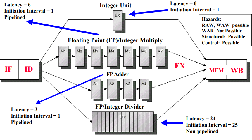
Instruction pipeline

The idea is to break up a single instruction broken up into multiple parts.

Each part executes in parallel with a different part of a previous instruction. Here is a diagram I pulled from the Wikipedia page on this subject.

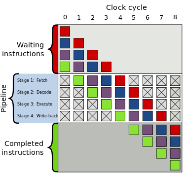
I will not use this particular pipeline as an example. Rather, I will use floating point pipeline as an example, as it is easier to demonstrate and more sensitive to software.

The idea is that there are many steps to executing a floating point number. The hardware designer can separate out these steps on the hardware, and leave locations to separate out intermediate data, then you can use every.

Here is a diagram from a really old presentation that shows this concept at a high level link.

Here is some very simple c++ code that multiplies a scalar by a vector of doubles.

1
2
3
4
5
6
7
8
9
#include <vector>
using namespace std;

void vector_scalar_mul(vector<double> & vec, double scalar){
    int vec_size = vec.size();
    for(int x = 0; x < vec_size; x++){
        vec[x] *= scalar;
    }
}

But this tells me very little on how it is actually executing on the machine. In order to learn more about that, I want to see the how the computer sees that code. It turns out that I am looking for the assembly code that the c++ code compiles to.

Luckily, gcc allows us to do this easily with a simple command:

g++ -S <file>

I want efficient code, so I ran it with

g++ -S -O2 <file>

You can try this out by going to this cool website (you might also want to click the “Intel” button to change the syntax to the same form that I am using here).

Here is a screenshot of this website:

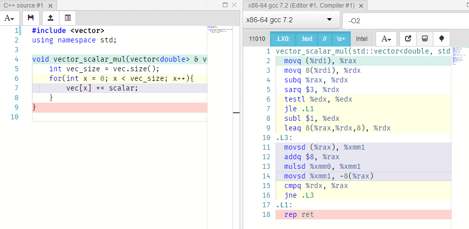
The generated assembly code is kind of messy, so I cleaned it up a little.

The important part is just the inner loop, which the online tool highlights.

mulsd	(%rax), %xmm1, %xmm0
addq	$8, %rax
movsd	%xmm0, -8(%rax)
cmpq	%rdx, %rax
jne	.L4

Now, this is how it looks to the machine. In order to get an evidence for how this is actually runs, though, we will need to actually run it, and measure how fast it runs.

In order to do that we need a little boilerplate code to run it a whole bunch of times.

1
2
3
4
5
6
7
8
9
10
11
12
13
#include <vector>
#include "pipelined_floats.cpp"

using namespace std;

int main(){
    int size = 1000;
    int iters = 1000000;
    vector<double> vals(size,1.0);
    for(int i = 0; i < iters;i++){
        vector_scalar_mul(vals, 1.00001);
    }
}

The only important thing to note about this code is that it runs the 6 instructions of the inner loop described above 1,000*1,000,000 times, or 1 billion times.

Now, how long should we expect this to take?

My computer runs at around 3ghz. According to intel’s documentation here, mulsd takes 3 cycles, and the rest of them take 1 cycle. So if this was executing sequentially, then it would take 7 billion cycles, which should take at least 2 seconds.

Timing the compiled code with -O2 using the unix time command, this actually takes a shocking 0.45s.

This means it is running more than 4 times faster than you might expect.

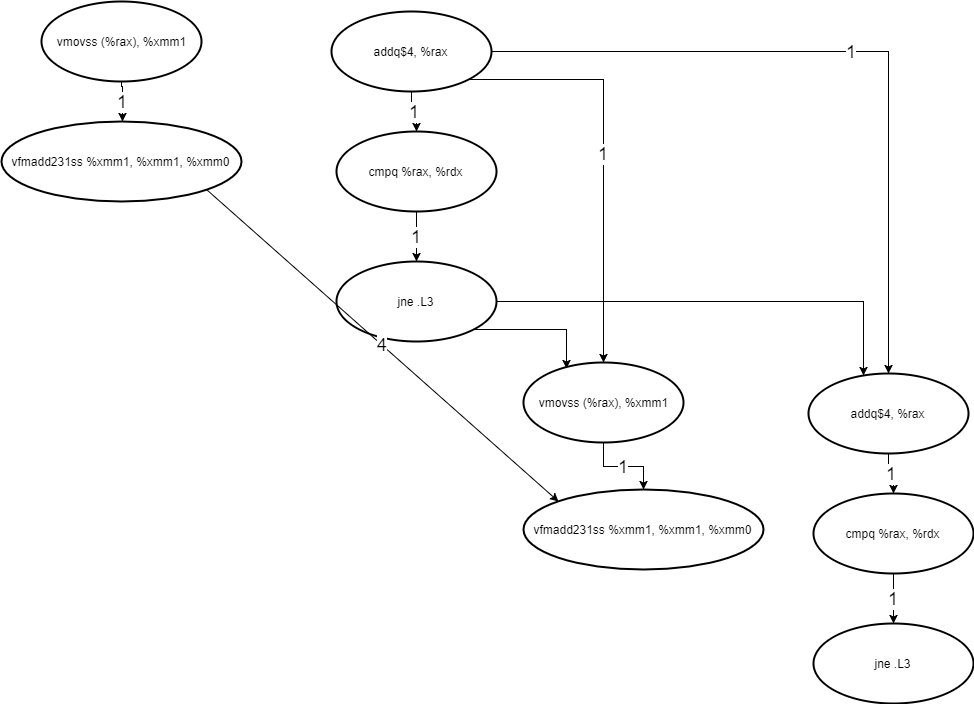
Here is an example in x86:

addq %rax,%rbx  // a += b

How does the pipeline interpret this?

LOAD (%rpi) //load the next instruction: "addq %rax,%rbx" from memory
DECODE // figures out if memory is

a