Guard-thief problem
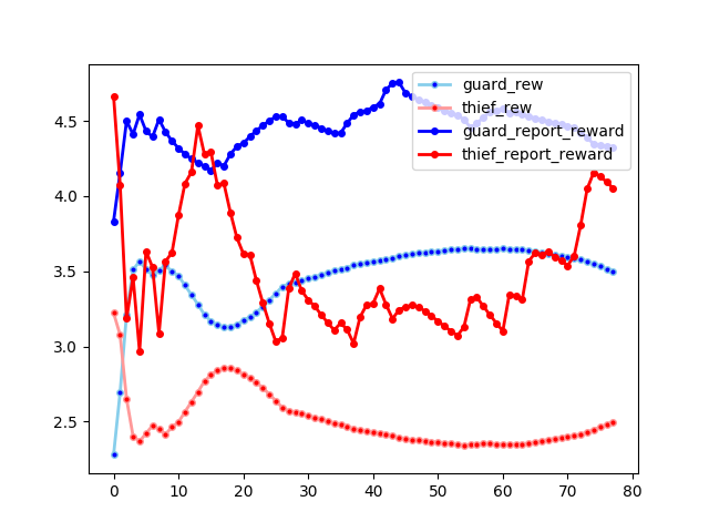
In graduate school, a result in a course project in a robotics class ended up changing my intended direction of study for the next year in a half, and completely changed my view of AI as a whole. This life-changing result can be summarized from a single chart: the learning curve below (solid lines are the marginals, light line are the means):
Ok, what is so exciting about this chart? Well, by itself, it could be any sort of issue with the learning algorithm. However, I had previously convinced myself, with extensive iteration and visualizations, that the code was doing what it should be doing, and actually learning good policies, and secondly, I knew from the literature that the algorithm in question was based off of a multi-agent population response method that was known to converge under weak assumptions. So, like every scientific discovery, the excitement was that one of these assumptions that looked pretty robust, was actually false in this case, and in fact, would likely be false in most circumstances which one would apply adversarial AI to.
So I was hoping to share the problem at hand and the reasons it is so life-changing.
Guard-thief problem
In robotics, there is a lot of asymmetric, zero-sum games which involve a guard which is protecting space, and a thief which are trying to avoid the guards, and find certain waypoints of interest. There are a bunch of different models of what kind of information each agent has access to.
- What line of sight does the guard have?
- Does the guard have to chase down the thief after seeing them?
- Does the thief already know the layout of the area and the waypoints they are targeting?
Game definition
After some iteration, the following set of rules were settled upon to make an practically interesting and tractable problem definition:
- The guard has limited lines of sight, blocked by both obstacles, and by distance.
- The game ends when the thief is seen by the guard, or when the thief finds all waypoints. The thief scores all the waypoints that were found before being seen, the guard is scored by the waypoints not found. (making it zero-sum)
- The guard and thief start out with perfect information about the scenario. (making it a planning problem, i.e. zero-information)
TLDR, its a patrolling problem, where the guard patrols the areas where he thinks the thief is likely to be at a given time-point, and the thief tries to approach the waypoints while avoiding areas where the guard is likely to be.
Practical motivation
The solution to this game can be used for stochastic patrol design. One problem with deterministic patrols (that is exploited so much in action movies) is that the thief can learn the patrol routes, and find gaps and weaknesses in them.
However, unlike in the movies, in reality, patrols need not be planned deterministically, rather, like rock-paper-scissors, the guard rotation can randomly choose from a distribution of patrols (even a small sample can be effective), and assuming the selection process is hidden from the thief, then the thief cannot avoid the patrol for certain, and must take calculated risks.
The guard is probably best off assuming that the thief is highly intelligent and highly informed, like the ones in the movies, and should model the possible thief as the worst case scenario, that the thief chooses the best possible route given the patrol distribution, and the guard should adjust their patrol distribution accordingly to account for this.
This intuitive iterative “Best response” optimization is the foundation of our solution methodology.
Example maps
Before getting to far into the methodology, I hope to show some examples of what this looks like. In the below visualization, there are 50 different samples of guard and thief paths being displayed on top of each other. In each simulation, there is only one guard and one thief, and the particular simulation ends when that guard and thief intersect, or when the thief finds all the waypoints.
Note that the different strategies the thief finds can be classified into different broad types of interpretable strategies.
- Speedrun: Running through the corridor, catching the waypoints as quickly as possible.
- Retreat: Pick up the first waypoint before retreating and picking up the second waypoint on the other side of the wall.
- Hide: Pick up the first waypoint before hiding on the outside of the building for awhile, before heading back in, hoping the guard is on the other side of the division.
And then sub-strategies of the above. The guards have their own counter-strategies:
- Protect: Rush over to the highest concentration of points at the back of the building and wander back and forth to catch any thiefs that approach.
- Cut off escape: The guard enters the building on the thief’s side, so that the thief cannot retreat.
But on some occasion, the guard is paired with a thief that it’s path never encounters, and so in 7 of the 50 simulations, the thief manages to pick up all 6 waypoints.
Note that the limitations of this map (such as the starting locations being fixed, and there only being one guard and one thief) are not needed for the optimization strategy below, which is powerful enough to accommodate variable starting locations or numbers without significant inefficiencies.
Game solution
A solid, efficient, effective solution, that improves with the more computation time you give it is essential, for both practical and scientific usecases. It is also not easy, and requires a variety of techniques in optimization, planning, game theory, and parallel programming. So its worth going into detail go into detail about how one solves a game like this.
At the highest level, the “Best Population Response” method is used for multi-player optimization. The idea is to calculate the best response for one player against to the existing set of solutions for the other player. Once that best response is calculated, it will be added to the population of strategies for that player. Further, we use a simple variant of where the opponents in the population are weighted uniformly, called Fictitious self-play. This method which was introduced by Brown, G. W. in Iterative solution of games by fictitious play (1951), and proven to converge to a unique minima in zero-sum games by Robinson, J. (1951) in An iterative method of solving a game. So after convergence, neither agent could benefit from switching strategies.
Best response optimization
Additionally, since the agents do not have any instance specific information about the other agents, they do not have to make any game-specific choices. This means that solutions do not need to have function policies that intake observations, instead, the policies are static, and can be parameterized by long paths through the map. I.e. a strategy is simply a path.
To find the best response path to an opponent, we can use a genetic algorithm, using the existing set of paths as a strong baseline set to start from.
To make this generic algorithm efficient, the genetic algorithm operates on high level target points, which an ordinary pathing algorithm converts into a continuous path. These target points are added, removed, shifted, swapped out, etc, in the mutation and crossover steps.
The scoring is done by checking all paths in the opponent population one by one. A single pair of (guard, thief) paths is efficient to check, simply by iterating along each timestamp and checking the respective visibility of the guard and thief for the victory conditions. With pre-computed visibility tables, a particular game score can be calculated in a few hundred CPU cycles. Some more details of the algorithm and implementation optimizations can be found in Appendix A.
Implementation
The full implementation can be found on github with some instructions in the Readme which can be used to reproduce the most of the plots and videos in this post. Map construction and pre-computation is performed in python, and the optimization is performed in c++.
Results/Discussion
In the above section we have determined that the agents seem to be discovering reasonable strategies, and seem to be producing a good mixture of good strategies.
Optimization Instability
Running the algorithm overnight, the unstable learning behavior at the top of the post emerges:
This is clearly not converging very quickly. In fact, it seems to be continuing to experience instability pretty far into training. However, the theory from Brown, G. W (1951) suggests that it should be converging, if we actually find the best response. However, we don’t find the best response because we are using an approximate optimization method with the genetic algorithm. So one of the key assumptions we pulled from the theory turned out not to be true. Furthermore, we are biasing the response by using the population of existing strategies to seed the genetic algorithm.
These differences between theory and practice give us two hypotheses:
- An imperfect optimization method, with or without bias, will result in learning instability and a sub-optimal strategy at every stage of learning.
- Any bias-free algorithm, even an approximate one, will converge, but perhaps to a sub-optimal strategy.
Zero-bias algorithm alterative
To isolate the effect of the bias, we can create an alterative algorithm without any bias.
Recalling that the bias came from seeding the next optimization step with the results from previous optimizations, we simply replace this population seed with a fully random seed. The following plot below shows the learning rate where each best response is sampled independently of the existing population response:
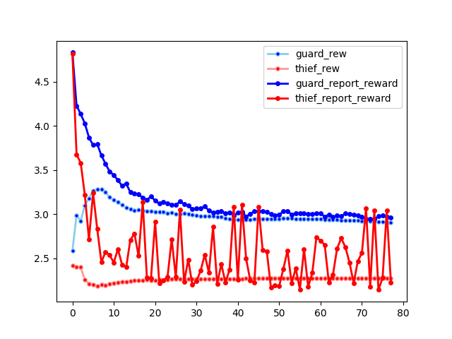
Note that unlike in the population seeded plot above, this plot shows fast population convergence. However, also note that the thief is having a hard time finding a best response, which is causing the spiky behavior in the marginal gain of the thief. Perhaps this could be solved by running the genetic algorithm for a much longer time, but that would make the computational complexity significantly higher.
Explaining convergence difficulties
This intrinsic difficulty in finding good paths for the thief, regardless of guard behavior, is also an explanation for the learning instability. It suggests that with or without biased seeding, the genetic algorithm will also struggle to find a novel best response for the thief. So if the genetic algorithm is seeded with the thief’s current set of paths, the algorithm might have great difficulty finding any better solution than one of the seed paths. This highly optimized seed path would then be added the thief’s strategy population over and over. You can imagine that the thief population might eventually start to simply sample from into, say, 4 highly optimized paths. The guard would then start to optimize to respond to that small set of paths, and would not take into account any alternative strategies. Then, if the thief finally stumbles across a novel strategy (perhaps hiding in a room for a few time-steps), then the thief would now have 5 paths to choose from, but the 5th path is so poorly represented in the population, that even if it is highly performing, it won’t budge the guard’s overall reward calculations until the thief samples this strategy hundreds of times. After which, it becomes a key optimization consideration for the guard, which might then sample a counter-strategy hundreds of times before the thief finally starts choosing the alternative strategies again.
The existence of persistent exploiting strategies
Observe another feature of the biased plot that is in need of explanation: the consistently large difference between the marginal returns of the newly added strategy (bold lines), and the average return of the population (shaded lines). Under convergence, we would expect that these two lines should converge, as the population reaches the nash equilibria, and it becomes impossible to find a better individual response than the population response. In the un-biased plot, we see a sort of approximate convergence, whereas in the biased plot, we see consistently greater marginal score than the average score.
This lack of convergence between the marginals and averages in the biased plot suggests that there is an exploiting strategy available to both agents at all times, but this exploiting strategy is heavily under-represented in their respective populations, due to sub-optimal strategies being selected over and over.
However, in the unbiased response, the genetic algorithm is unable to clone old strategies, and so there is no cause of a delay between the population set and the marginal response, so the marginal and average lines do indeed converge quickly, as there is no exploiting strategy which can be accessed and copied over and over again.
Is bias or variance more important overall?
To any pragmatic mind (including my professor’s), the question of “well which one is better overall: biased or unbiased response”, is the first thing to ask. Unfortunately, this is a difficult question to answer in general, as it depends on the relative difficulty of responding to the other agent’s choices, vs the difficulty in achieving adequate results in one’s goal independently of the other player (i.e. the thief has to actually find the waypoints).
However, for this particular guard-thief setup, it shouldn’t be hard to answer, just run the strategies each method uses against each other to get a score. I didn’t get around to this particular task, but does this capture your imagination? Would you be interested?
Appendix
Appendix A: Implementation details
So, in pseudo-code the algorithm is simply:
thief_paths = [random_path()]
guard_paths = [random_path()]
loop
    seed_thief_paths = [random_path()]*10 + random.sample(thief_paths, k=100)
    for i in range(GENETIC_ITERS):
        seed_thief_paths = crossover_mutate(response_thief_paths)
        thief_path_scores = population_response_score(seed_thief_paths, guard_paths)
        seed_thief_paths = filter_by_score(seed_thief_paths, thief_path_scores, count=100 if i != GENETIC_ITERS-1 else 1)
    thief_paths.append(thief_path_scores[0])
    # same thing for the guards
Additional important optimizations include:
- Pre-computing the visibility function of the guard, so that the question of whether the guard can see the thief at a given timepoint is a simple table lookup.
- Pre-computing the thief’s capture space so that the thief finding a waypoint is a table lookup.
- Parallelizing the NxM
population_response_scorestep using OpenMP. - Parallelizing the
crossover_mutatestep.
Appendix B: More results
So you can get a better idea of how training progression works visually, here are a full sample video from different steps in the population accumulation process. You can observe that as learning continues, more different sorts of strategies are added to the set, and occasionally some strategies lose importance as the opponent adapts to them, and no longer appear in our sample of 50. However, remember that no strategy is completely forgotten in Fictitious self-play; all historical strategies are weighted equally when computing best responses.