Intuitive introduction to improving RNN models

Creating long term memory for a neural network

Code and data here: https://github.com/benblack769/NNetExperiments

Introduction

Assumed Knowledge

Now, to start off, I am no expert in neural nets. I spent a month or two learning about them from excellent sources like this.

If you have a good understanding of linear algebra and multidimensional calculus, you should be able to pick it up quite quickly. But neural nets do not use super advanced mathematical concepts, so don’t let the math scare you too much! You should be able to learn the math alongside the network specific info. Why am I going over this? Because for this post, I will assume some basic knowledge about neural nets. I will assume you have a decent grasp of gradient descent and of ordinary three layer neural networks. There are already a million great sources to learn the basics, and far too few going over more advanced concepts.

Inspiration and Goal

One thing to know about LSTMs is that they are invented in 1999, and are still by far the best general purpose time series predictor known. This is not due to a lack of effort. There have been advances in

• Mathematics: Hessian free optimization, an effective second order optimization model, has been successfully applied to neural networks)
• Neuroscience: We have a much better idea of how neurons actually interact) Recurrent neural network design: Inspired by LSTMs, many people have created similar models which they though would solve some problems that LSTMs seem to have. None of the dozens of these are substantially better, although some are marginally simpler. A meta-study done recently found that some models are marginally better.
• Augmented networks: Many people think the next big thing in neural nets are ones given external memory to work with. These are often combined with LSTM networks to solve some of the most important pattern recognition problems. Google’s new translation algorithm uses Attention networks to augment LSTMs.

So what makes these so powerful? What made people think they could be improved with minor changes, and why were they wrong? What can’t it do? If we ever want to make something even better, perhaps solving some of the problems with LSTMs, we need to be able to answer these questions. I think that LSTMs might encode something fundamental about intelligence, although it may not be easy to see what that is.

Recurrent Networks and Time Sequence Learning

First, what is a recurrent network? It tries to solve a common problem that humans solve, which is recognizing sequences over time. It does this by looking at the data one timestep at a time, only storing a fixed amount of data from previous timesteps. For example, RNNs are used for voice recognition, i.e. turning a sequence of sound waves into a sequence of letters.

A recurrent network broadly it looks like this:

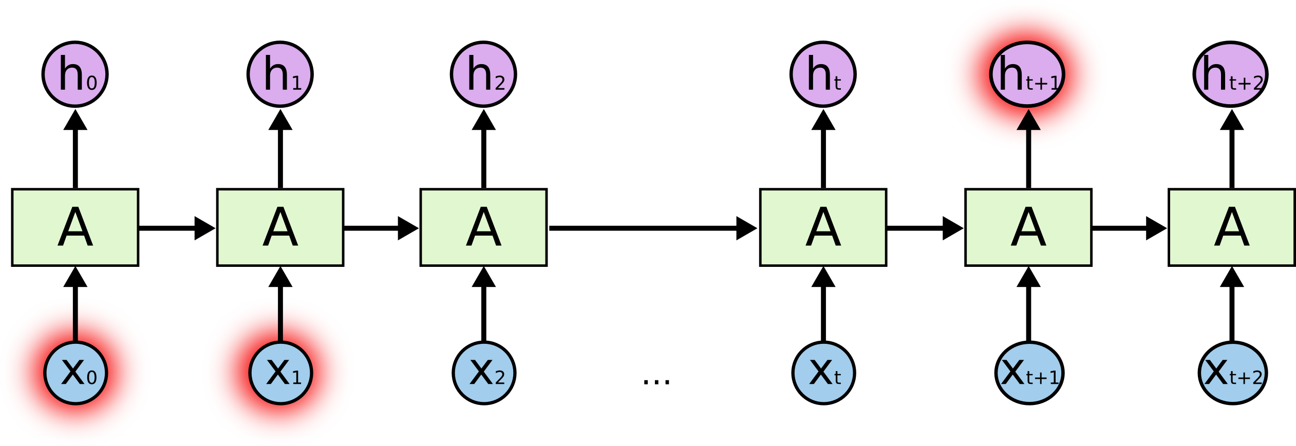
The major parts are the input, a state which is a function of the previous inputs, and the output, which is a function of the previous state. For voice recognition, the input would be some representation of sound waves, and the output would be text. In order to train the model, the output would then be compared to the expected output, which is usually computed by hand (by writing out the text that the person is saying). Then, as long as the function A is differentiable, we can use backpropagation with gradient descent in order to get it to learn. I’ll explore gradient descent in more detail later.

So how do we construct such a function so that we can nicely change the parameters like that? The obvious construction follows directly from ordinary deep neural networks.

Description of ordinary recurrent networks

Traditional RNNs are built as follows:

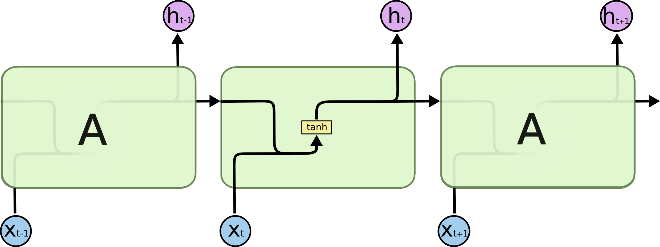
As you can see, there is a state which propagates through the network. You can imagine that with every timestep back, you are going back another level of depth in an ordinary network. In real implementations, there is another layer before the output. So the input in the same step is a 3 layer network, the step before is 4 layers deep, etc.

Why ordinary RNNs fail

The problem is that this is simply too deep. At least with ordinary gradient descent, you run into the dreaded vanishing gradient problem, where each input effectively affects each output in a more and more uniform way as the network gets deeper, so there is less to learn. After 10 or so layers, it is basically impossible to learn anything at all. This paper goes in more detail about why regular RNNs simply do not learn longer term dependencies (longer meaning more than 4 or 5).

Description of LSTM networks

Colah’s blog post here is a great description of the structural aspects of LSTMs. I will cover a little of what is there, but not everything. I will be using diagrams from that source (which are generously published as public domain).

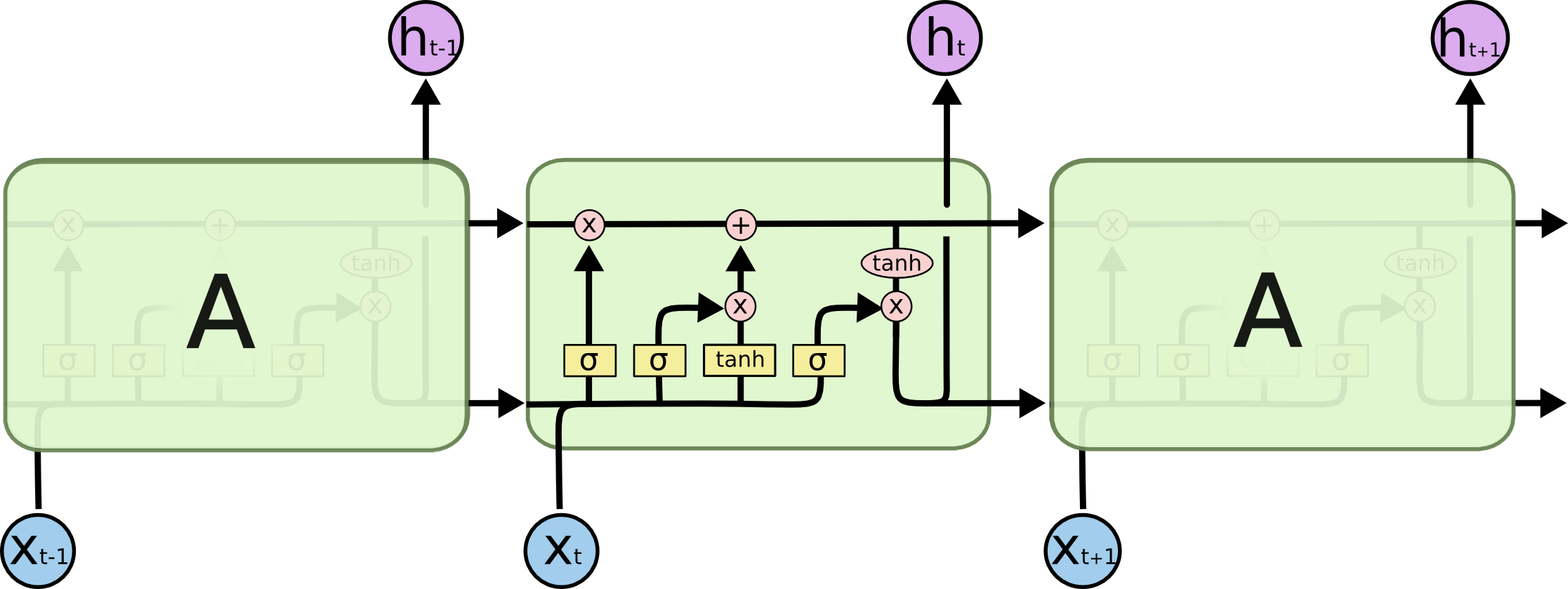
The primary intuition behind this is that the cell state (the black line on top) is the information that is held from previous states. It is multiplied to by a number between 1 and zero, “forgetting” previous knowledge. It then adds to that cell state, “remembering” current knowledge. Its output is then some filtering of that cell state (which is why there is also a layer in between the output and the actual output in a real LSTM).

In terms of depth, it has aspects of both deep and shallow learning, which is what makes it so powerful while still able to learn long term dependencies.

The reason why it doesn’t have the vanishing gradient problem as badly as traditional RNNs is that the single cell state is only changed by a scalar addition and multiplication, rather than multiplying the value by an entire vector and adding it to the next state. Intuitively, information is simply flowing through the cell, only changing by a little bit, rather than being fundamentally recalculated at each time step. So long term data is handled similarly to a shallow 3 layer network: Data that is added in one time step flows directly to the output, with the only other thing affecting the data is just reduction of its magnitude.

The deep part is how the output, which is a filtering of the cell state, is joined with the input, and is used to determine what things are forgotten, added, etc.

Actual Implementations and Some Results

First Neural Net

To get back into practice with neural nets, and accustomed myself to the working of Theano, I made an extremely simple 3 layer neural net, and trained it on an extremely simple learning task. The task was to learn a Caesar cipher of 1, that is the letters A,B,C,…,Y,Z turns into B,C,D,…,Z,A. Even though this is a trivial learning task, it reveals some interesting facts about neural networks and gradient descent.

The data set I was training on is an excerpt from Douglas Adam’s Hitchhiker’s Guide to the Galaxy. It is in data/test_text.txt. The code to run the learning scheme is in theanoexp.py. It encodes the letters with a 26 node input and output, which correspond to the 26 letters, and has a hidden layer size of 100.

Random initialization bug

When I first wrote it up, I had the problem where it would always output the same random letter, no matter what training occurred. I eventually figured out that the random weights and biases I initialized the matrix with were much too large. Just an example of one of the ways ANNs depend on values to work, not control flow.

Unstable Biases

I used my tool to get the biases as they were training to see if they eventually stabilized. The following records a selection of the hidden layer biases 300 cycles through the text.

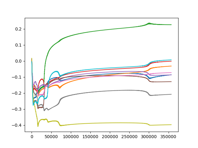
As you can see, it does not seem to stabilize perfectly, even over hundreds of iterations over the dataset. Instead it seems to slip every once in awhile into a new sort of state. This is an interesting phenomena, which suggests that the gradient descent is actually operating in a relatively complex space with local critical points. This is counterintuitive considering the (input, output) pairs are a linear function, and so it has no local optima. The cost is quadratic, not linear, but it also has no local optima. However, note that the neural network itself is not a linear function, and the weights are not updating in the space of the inputs and outputs, but rather in the space of the parameters of the NN and the cost And so we learn that the parameters are interacting in complicated ways even in this simple learning task.

To me this is reminiscent of a human learning a simple tasks. I have a hard time learning the Ceaser cipher in such a way that I can get in letters and immediately spit out answers. Even after doing it for awhile, I still sometimes makes mistakes. I can overcomplicate and overthink simple tasks like this. This is interesting because even on tasks where neural networks are not the best type of learner (a linear learner would be better), it still seems to mimic human learning.

Optimizers (RMSprop)

First, a quick overview of the history of ANN optimizers:

http://sebastianruder.com/optimizing-gradient-descent/index.html#adadelta

Gradient descent has many well studied mathematical problems. It gets stuck in local minima, it can bounce around between the sides of a valley before coming to a rest at the bottom, and other problems. Attempts to come to a solution have often been too slow, or not generally applicable. The evolution of these has accumulated in three general purpose optimizing algorithms, Adam, AdaDelta, and RMSprop. All of these have slight alterations to the basic gradient descent which try to intelligently pick the size of the step. I implemented RMSprop because of its simplicity and power. Amazingly, this widely used and generally admired optimizer was first introduced to the world through some slides on a Coursera class (link).

Description

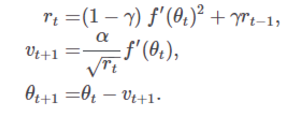
Here is the actual formula that is used to calculate it:

Gramma and alpha are parameters that you get to pick. gamma is usually around 0.9. Theta is a measure of the magnitudes of the previous gradients. In theory, what this does is make the learning rate smaller when the gradient is steeper, perhaps slowly lowering the values into a “canyon” (where normal SGD will overshoot the valley of minimal loss and end up on the other cliff). It will also make larger changes when the gradient is smaller, which can help it get out of local minima.

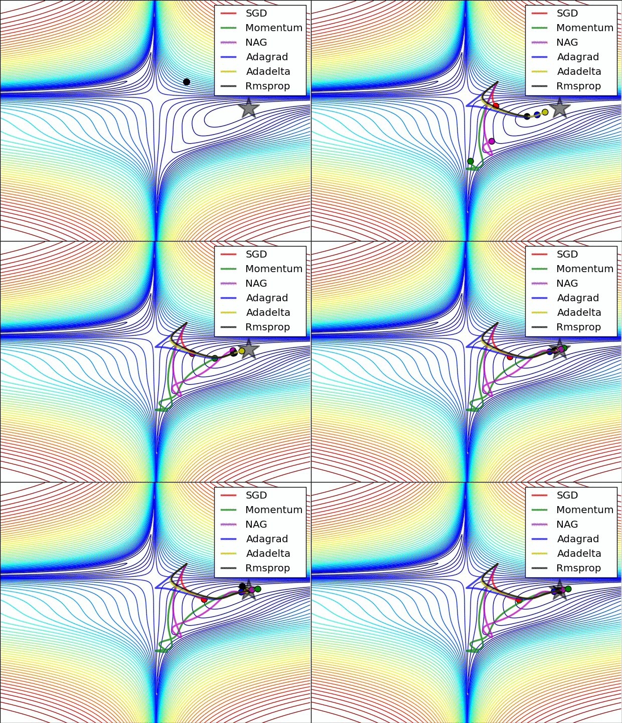
This great blog describing this problem in detail built some small dimensional visualizations to capture this intuition, and show how it performs in comparison to other approaches, like the momentum approach.

This one shows an example of how momentum approaches can do worse than RMSprop and AdaDelta.

This one shows how RMSprop can get out of an unstable equilibria very quickly.

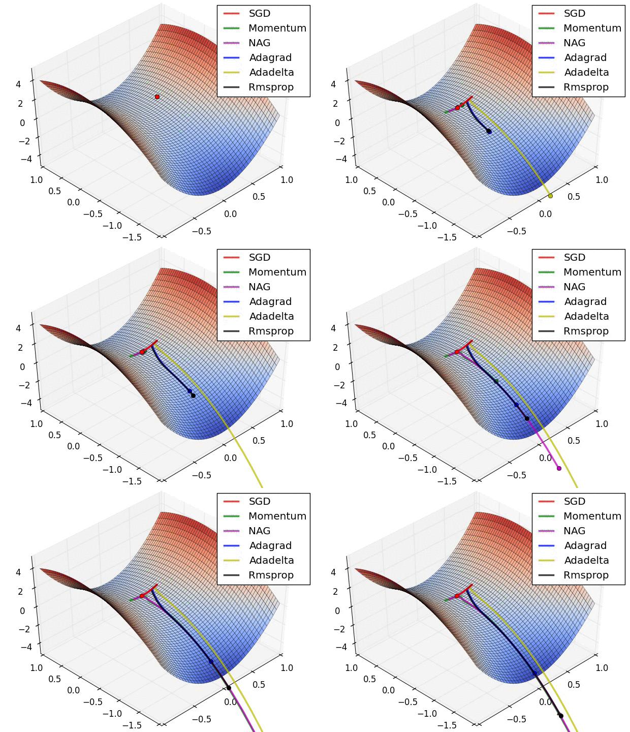
However, these are contrived low dimensional problems. We want to know if these things actually work on extremely high dimensional neural networks training on real problems.

In order to see if this stabilized anything, I went ahead and ran it, capturing the updating biases as it updated. Ignore the x axis, this chart is on the same sort of timescale as the one above using ordinary SGD.

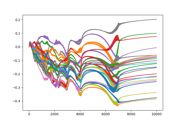
You can see that at the very beginning, it is changing much slower than SGD. This is almost certainly the primary intention of RMSprop: to stabilize outcomes by forcing it to change slower so it doesn’t jump to some horrible state when updating. However, it is not so clear that it always works better since sometimes you really do just learn the easy stuff to learn as quickly as possible.

Since this learning task is so easy, I expect it to actually performs worse on this learning task (or at the very least not much better). This is because the space is so simple, it is OK for SGD to update quickly at the beginning. So all RMSprop does is slow it down. The space it is optimizing over is not nearly complex enough to need it. However, I did not have enough time to verify this using real data.

The fact that in actual learning tasks, RMSprop and similar methods are so popular seem to indicate that in real learning tasks, steady learning processes are essential for gradient based learning to work.

We do not think of ourselves learning steadily, though. When we see something surprising, something wildly different from the norm, we often focus on it, and think about it a lot. RMSprop ensures the opposite, that when something is encountered that is different from the norm, the total amount the ANN learns from it is in fact not much greater than what we expect to see.

To me, this suggests that RMSprop is simply operating at a different level than what we think of learning in humans.

Instead, it seems to be more similar to how humans experience sensation. When we have more inputs: our eyes are open, we are seeing lots of bright things, listening to loud music, etc, then it is harder to focus on smaller details. Only the most extreme sensations stand out.

Sensation and learning do not really seem to be innately related. In fact, they are in a way fundamentally different: RMSprop’s optimizer has to do with regularizing outputs, and sensation has to do with managing inputs. However, I still think RMSprop and the human adjustment of sensation are solving a similar problem: that just because there is more to see, or more to learn does not necessarily mean that it is that much more important.

LSTM

Learning task

I will start out with a rather simple learning task: recognize most likely next letter.

For example, if it gets input “I am goin”, it should output “g”, as it is pretty obvious that the statement is: “I am going”.

One nice property of this task is that if you know English, you should be able to perform the task better. So perhaps in order to perform the task, it also will learn a bit about English in the process.

Training text

I chose the text Huckleberry Fin, partly because its copyright is expired, and partly because it has a distinctive writing style that we can see if the network identifies. I found a text copy on Project Gutenberg (license)

Initial results

I trained this using a network with cell states of 200. Afterwards it matched text like so:

Top text is original, bottom text is the guessed next letter. To see how it performs, you should look at the previous letters and see if you can guess what the next letter would be just from those. Then see if the machine guessed it.

As you can see, it tends to simply guess spaces, and ends of common words. At the beginnings of words, and in less common words like “adventures” it does very poorly. Overall, the results are not particularly impressive. I ran it on the whole text, and it only guesses 54% of the letters correct. Comparing this to standard compression algorithms, which can compress ordinary text into 1/8 of the space without any knowledge of the language, this is pretty bad.

So why might it be relatively poor? There are many practical reasons. For example, my network may have not trained fully, 200 cell states might just be too few, etc. But before I go over that, I would like to look at exactly how it trained.

Visualizations of the training

Here is a typical view of how the error updates over a long period of training.

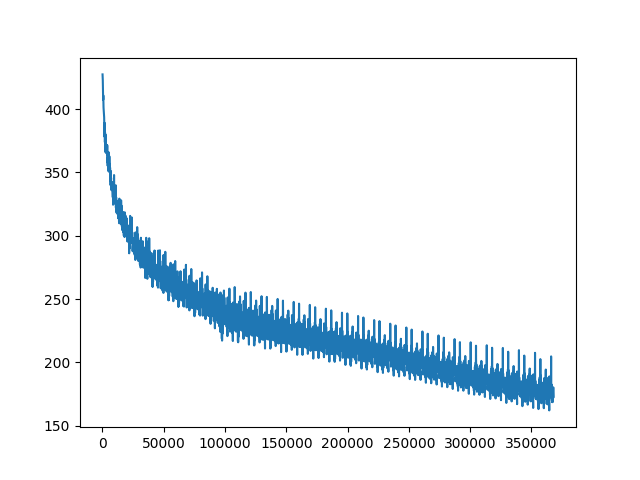
There are three main stages I observed. The first stage, there is very quick learning. Then, it stabilizes to almost completely linear cost decrease. Then it goes on like that for awhile until it eventually flattens out. I saw this in almost every plot of error for the “guess the next letter” task.

The part where it becomes almost linear is deeply confusing to me. Part of it might be the effect of RMSprop increasing the learning rate if the error decreases, but even still, I feel like learning should be more similar to exponential decay than linear decay. After all, surely if you learn a little it is harder to learn more.

Experimenting with the learning parameter a little, and increasing causes it to stop learning at all (the cost will actually increase a little, then stabilize), and decreasing the cost will just make it learn at a lower linear slope. I am not sure what to read from this linear behavior of training, but it is a curiosity. Perhaps it is related to the structure of LSTMs somehow. I have a suspicion it might have to do with the way the forget gate can only learn things if the previous add gates have already learned things, which then allows those add gates to learn more. This definitely warrants some more investigation, but I do not have time here to explore it comprehensively.

Standard improvements

So if the result is poor, then there are many ways people like to introduce which may help the LSTM.

• Dropout and/or regularization
• Fiddling with learning parameter (particularly lowering it, and training it for longer)
• Layering multiple LSTMs on top of each other
• Many others…

Unfortunately, I will only explore the 3rd option, layering. It seems like the most important, and most likely to seriously improve my network.

Deep Layering

So my next attempt to make this better was to layer two LSTMs on top of another. I also made the cell states larger, to around 500 for both layers.

Unfortunately, after 3 days, it still did not really finish training, as you can see from the error not stabilizing:

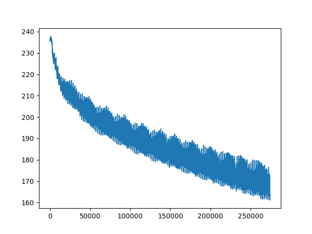
As it did not learn fully, it did not reach the levels of the much simpler networks, only guessing the right letter 49.7% percent of the text correctly. To me this exemplifies the tradeoff with deeper networks: it might work better eventually, but it also may take forever to learn.

LSTM Part 2: improving the network

Why try to improve the network?

Unfortunately, it is difficult to test theoretical hypothesis of how LSTMs really work. We know they work, and we can state properties of them, but especially something as complicated as LSTMs, it is hard to concretely track down any sort of causation or fundamental nature.

However, if we can show that certain intuitions consistently describe how various kinds of networks operate, then we can be more confident that they have some meaningful value. However, there is a little bit of a problem because it is easy to find consistent features in existing NNs, and base intuitions that condense already known information. However, it is unclear weather these are informative truths, because there are many intuitions that can describe known phenomena which are completely wrong. So instead, I will try to use my intuitions to create a new sort of network. In particular, I will explore how one might improve LSTMs, and suggest some improvements. If those improvements work, then that gives some evidence that my intuitions about RNNs are correct.

This would not be particularly strong evidence. Perhaps I gained some knowledge which I did not communicate in this paper, and that is the knowledge that allowed me to improve the network. This is unfortunately rather likely: talented neural networks developers consider ANN improvement more of an art than a science. But I don’t know a better way, and I do think it is better than what people tend to do, which is just condense down things they already know work.

Model 1

My first attempted improvement tried to see if one network can learn something about the broader aspects of language.

Inspiration

Attention based networks have made significant strides in time sequence analysis, such as translation. But current methods are inefficient for long time series. One potential goal of a lower level network model is to condense the important information in a long time series into a relatively small number of steps, each of which containing a reasonable amount of information. In other words, to compress the time scale of the data, without hugely increasing the spatial scale. It is not clear that current techniques like layering LSTMS do this efficiently.

I think that this condensation over time is vital to creating human level intelligence. The very idea of attention is related to the conscious self, which can only focus on a small number of things at a time. So it relies on something lower level to condense the relevant information to something we can reasonably expect the machine to focus on.

Description

Basically, I want to see if we can use the cell state of a network which is performing the learning task in order to make another task learn better or faster.

But what do I mean by “use the cell state”? What I worked out is that we can build another LSTM which tries to predict the next cell state of the other model. So I have an LSTM which can understand the nature of the other LSTM.

Then I can use a third LSTM to learn from the output of the second and the original text in order to learn the task faster or better.

My results were that the 3rd LSTM actually did learn much faster, but not substantively better than the first (both had 200 cell states).

Try comparing the two plots below, the first is the 3rd LSTM, which takes in input the one that understands the first LSTM, and the first LSTM. They both have identical parameters for everything else.

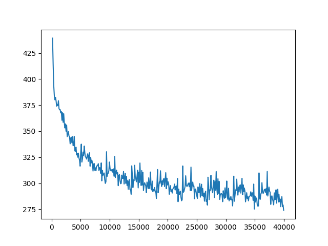
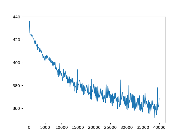
As you can tell, the 3rd LSTM actually learns much, much faster. In fact, the it stabilizes completely at around cost=260, whereas the first one very slowly declines to around 270.

It also classifies slightly better, at 57% of letters guessed correctly rather than 54%. But since I didn’t train to exhaustion, this may just be a result that it learned faster (although this highlights the fact that in certain circumstances learning better and learning faster are pretty much the same as time is restricted).

In hindsight, I am surprised this approach worked as well as it did. It also became clear that this model cannot possibly become better than the original, because the second LSTM can only learn what the 1st one is doing, so it cannot actually help improve upon it. So the third layer can’t possibly do better than the first.

On the other hand, the fact that it trained so much faster suggests that the second layer really did learn something important about how the first one operates, information that another neural net can easily use.

The next step in this exploration would be to see if the 3rd layer can be replaced by another layer which instead of trying to guess the next letter, performs some other learning task, such as trying to calculate the part of speech of the word (it would only output anything at the end of each word).

While I did not have time to execute this and see if it works, I suspect it will. If this is true, then I have successfully condensed down some information about english into a form more easily processed by LSTMs than raw letters. I would say that this is the machine abstracting, condensing, and packaging english. Perhaps this way it can behave like humans do when we learn a task faster the second time, or learn a similar task faster.

If an LSTM on another learning task does not work, then it still shows that the cell state contains some infromation that can be used for something, even if my particular model did not work very well.

Conclusion

In this attempt to try to understand LSTMs, I learned that there a number of important parts to them.

• The algebraic structure of how the output is generated.
• Gradient descent, and the optimizer which tries to make gradient descent work better.
• The way the weights are randomly initialized.
• The cost function
• Depth of the network and how that depth affects learning
• Hardware performance and batched learning

All of these have been studied in quite some depth independently. In my attempt to learn and understand everything at once, I went a little over my head and failed to get decent results for some of the more difficult experiments at the end.

However, by studying them all, I encountered some consistent themes.

First, In the history of ANNs, there are two main approaches to developing techniques to solve current problems with ANNs. The first is to use ideas inspired by neuroscience and by human phycology. The second is to use more mathematical structures and ideas to solve those problems. One of the things I found is that these approaches are not mutually exclusive: Ideas with more mathematical origins, like RMSprop, can have human interpretations. And of course those with more neurological origins, like attention, can be studied using math.

Second, LSTMs are hard to work with, and even harder to improve. Training takes forever, and even with careful thought and observation, keeping parameters nicely tuned and the network training smoothly is time consuming and difficult. And even when parameters are really good, it can still take a day or more of training to get it to work even remotely well, far more in some cases. According to my calculations and timings, my bigger networks were calculating at 60 GFLOPS, about the computational power of the Deep Blue chess computer. This is well below the theoretical capacity of my hardware, but it still seemed pretty good to me, so it was not just my code being slow. In a practical sense, this explains why neural networks are not yet used for everything, and why so few organizations are willing to try cutting edge ideas. In a more theoretical sense, it showed me that these techniques are really stretching the boundaries of current hardware. I now understand why DeepMind, and others put so much effort into configuring large hardware system to run their networks on: to get training to happen in a reasonable amount of time. The fact that training was so frustratingly slow, even on decent hardware, made me think one of the following is true:

1. Perhaps gradient descent is actually suboptimal and there is actually a better way we haven’t discovered yet.
2. These tasks are fundamentally quite difficult to learn, and our brains are simply incredibly well suited to learning these sorts of tasks.

Note that these are not mutually exclusive. But the second one suggests that significant hardware advancements might be necessary for machines to truly reach human level ability.

Third,

Appendix A: Thoughts on Debugging Neural Networks

Now, when people show you their neural network code, you go off, and try to run it, and it may work, but good luck making any changes. Neural nets are notoriously tricky. Out of all the code I have ever written, they have the greatest barriers to debugging. The code will run with several major errors, but it will not do what you want to do without everything being perfect. This is the case because there are no conditionals in the main part of the code. You can write out just about every ANN ever invented without loops, if statements or recursion. This is not only speculation or theory, some code I wrote does just this, outputting code without loops that computes a simple, but practically useful neural net (see my Graph Optimizer project for more details). What this means is that every part of the code is important to every part of the computation. There is not any part of the code which is not run for certain problems.

I this is an interesting contrast to standard AI techniques, which may be fiddly, but if you make one minor error in the code, then usually most things work fine, or it crashes immediately, or at the very least, it is easy to trace back what exactly went wrong. In general, it is easy to debug. This is because for GOFAI, we are navigating around some sort of finite state machine, or some sort of symbol processor, or decision tree, or something, and in all of these, we can think about the program moving around, doing different things in different cases. This is the case because the symbolic concepts of the AI tend to be directly correspond to exact lines of code, or at least a fairly small section of code.

I believe that this difference between GOFAI and neural networks is interrelated to the difference between symbolic and sub-symbolic computation. This suggests that while sub-symbolic computation poses many solutions to philosophical and computational problems, it poses an engineering problem: how do we examine a bit of code which every part, every piece of data affects every other part?

Solving this problem requires new debugging tools, new tests, new debugging thought processes, and maybe even new hardware. Instead of thinking about an instruction pointer going around, we need to think about data changing, its interactions with data around it, how it accumulates, increments, and compounds. We need visualizations which allows us to see how the data is changing, not which instruction the computer is following.

My solution was to create line graphs that displayed certain values over time. Many of those graphs are above. In order to do this easily I made a simple tool that save values in the network to a file (plot_utility.py), and a tool which uses MatPlotlib to create a visualization of that data (plot_data.py).

However, this is admittedly a deeply imperfect solution, as these line graphs only display a small fraction of the data, and not too clearly at that. It is also extremely difficult to see how they are interacting. Causality is completely confounded. This makes my plots not as useful as I hoped they would be. However, I believe that there are better ways out there to look at the real computation happening inside the data.

Appendix B: Execution and Debugging of Neural Network Code

Theano

Ok, now on to creating the code. I chose Theano, which I think is a really cool framework, independent of all the cool neural networks it allows you to build. Basically, it view the program as a graph. This allows the following:

• Manipulate the program graph in order to make the code faster.
  • memory reuse optimization
• Hardware support
  • Very easy and efficient GPU computation
  • cluster computation, including muti-GPU computation
• Allows for easy generation of code flow charts
• Automatic and efficient computation of gradients, saving a lot of code

Unfortunately, it comes with the downside that the code creation and execution are more separated than usual, making it somewhat harder to debug. Luckily, the Theano developers put a lot of work into making this problem better.

Saving/loading of trained weights

Training takes awhile. At least when I did it, I wanted to stop the process so that I could view plots, adjust learning rates, and see if it is actually learning. I then wanted to start it up again right where it left off. The shared_save.py file is dedicated to this task.

I found this absolutely essential to effectively working with this experimental work.

It also was nice because then I could use Amazon Spot GPU instances, which are much cheaper than On Demand instances, but can interrupt your code at will.

Batch Learning

The primary hardware optimization for Neural Networks is batched learning. Some people mistakenly think that this has some deeper meaning which it does not (batches of size 1 are optimal for sequential processors), but it does allow significant data parallelism. It makes the difference between GPUs being useful and useless, and even on CPUs makes it many times faster. I used batch sizes of 128 or 256 on GPUs, which allowed my model to train dozens of times faster.

GPU install process

It turns out that installing all the software for GPU computation using Theano is amazingly hard, at every level. CUDA, which Nvidia puts substantial amount of effort into making installation easy, requires the unbelievably bloated VS 14 compiler on windows, and substantial system configuration on Linux. Theano’s gpuarray backend is broken on windows and you need to install from source on Linux.

Basically, if all this installation process was easier, people would use GPUs much more for computation, and probably deep learning as a field of study would be more accessible.