Fast, Simple, Effective Rectangle coverage

Rectangle coverage

The inspiration for this problem comes from a real world challenge I encountered when translating human object annotations into inputs for a deep learning system at Techcyte. In this business, domain experts review gigapixel whole slide image scans, and box interesting objects that they find. They are instructed to only label exemplars, that is, the clearest, most distinct objects, and they don’t worry about comprehensive labeling. However, small objects are often labeled in the same general area of the scan, for convenience of the human annotator, so there are sometimes many annotations grouped together.

Neither humans nor standard deep learning systems can examine gigapixel images in one go—the task must be broken up into smaller tasks that can fit into memory. Typically, this is done through simple tiling strategies. However, since since annotations are not expected to be comprehensive, the deep learning system’s loss function is customized to ignore all unlabeled objects during training. So tiling unlabeled areas is wasteful. And so efficient tile generation becomes a covering task, where we wish to generate tiles which cover all the areas of the image where there are human annotations, and to ignore all the areas which there are no human annotations. Furthermore, our object detection problem is easier if each object is fully contained within the scene. So we require full containment as a constraint.

We can reduce this to an abstract constrained minimization problem as follows: Given a tile size of (X, Y) and a set of boxes {(x, y, w, h)...}, we must generate a set of tile coordinates such that every box is contained within at least one tile, and within those constraints, we hope to minimize the number of tiles.

A sneak peak of the algorithm in action is shown below:

Analogous problems

This algorithm has close relationships to two better known algorithms:

1. Set-cover (Given a bunch of sets of elements, find the minimal selection of sets so that you get every element)
2. Radial cover (think covering an area with radio towers)

Set-cover is a nice analogue because our problem can be directly reduced to it. In our problem, the total set you want to cover is the set of all boxes. The subsets you wish to select from are the tiles which contain them. Unfortunately, set-cover is known to be NP-hard

The NP-hardness of set-cover should give us pause. Even though the geometric limitations of rectangular cover means that it might not be NP-hard, this correspondence to set-cover means that it will still likely be expensive to compute an exact solution. Note that radial cover problems are also generally fairly hard to find exactly optimal solutions to.

So we can turn to approximation algorithms with a good conscience that we are probably not passing by some efficient exact solution. Set-cover is known to have a simple, and fast approximation algorithm: Greedy selection. In our language, greedy selection means simply choosing the tile which covers the most so-far uncovered objects, removing those objects, and repeating. Unfortunately, this greedy algorithm is known to have a worst case bound of O(log(N)). Even worse, it is a tight lower bound for polynomial time algorithms: set-cover has an inapproximability result that states that simply achieving better than O(log(N)) is also NP-hard.

While again, it is unlikely that this inapproximability result is valid in the 2d case, you can construct some pretty bad examples of the greedy algorithm for our rectangular cover problem.

For example: Take the following arrangement of blue boxes, and the following simple green tiling that produces the optimal solution of 4 tiles.

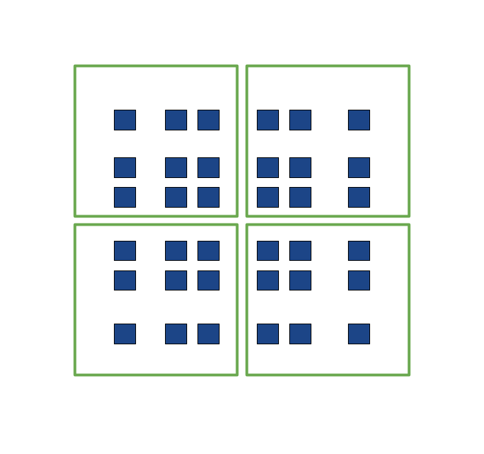
Now, consider that the greedy algorithm will start with the densest area in the center and edges, and work its way to the sparser areas on the corners, generating this 9 tile solution.

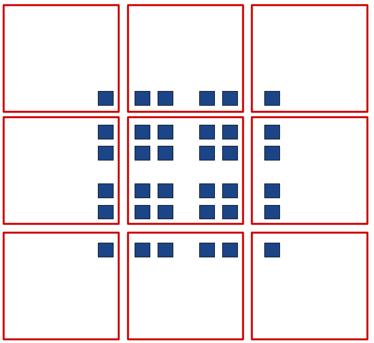
So at best, the greedy algorithm is a 9/4=2.5 approximation. Which isn’t ideal. It is also a bit tricky to implement this global greedy algorithm efficiently, as there are many possible candidate tiles to choose from when trying to find the globally best tile each iteration. However, it does have the same theoretical bound as set-cover, and it also raises some interesting implementation challenges.

Geometric analysis

It would be interesting to explore alternative strategies which utilize specific geometric properties which allow for better approximations than set-cover with simpler, faster implementations. However, we are pragmatic people not geometry wizards, and the greedy solution isn’t bad, so instead of beating our head against the wall, we can just try to find efficient implementations and heuristics for the greedy solution, and see if we get any useful geometric insights.

Four questions inspired by global greedy idea

One good question inspired by the greedy solution is: Question 1:, How would we go about finding the best single tile that covers the most boxes in a scene?

Well, one way to do this is to narrow down all the possibly optimal tiles to a finite set and check them all. Giving us a new problem, Question 2: How can we enumerate all possibly optimal tiles?

To start, consider this set of boxes and associated tile:

Notice that this tile can be shifted around by a considerable amount without changing which tiles it includes. It can be shifted even more if we allow it to include at least all the same tiles it started with, and possibly more.

To reduce the set of possible tiles so can hope to enumerate all of the possibly optimal ones, we should try to normalize each tiles to a similar tile that includes at least as many objects as the original.

Raising Question 3: How can we take any given tile, and generate an equivalent, easily defined tile, that includes at least as many boxes?

Well, one simple way would be to shift the tile down and right to the very edges of the left-most and top-most boxes contained in the original tile, e.g.

And you end up with a tile which contains at least as many boxes as the original. Answering Question 3 quite nicely.

Since all optimal tiles are equivalent to a tile which has a left-most and top-most object, we can construct a set of possibly optimal candidates by simply considering all top edges and left edges of all boxes and their respective tiles, eliminating invalid tiles. This operation is O(N^2) where N is the number of boxes. This is already polynomial, a good start to Question 2. But N can be in the hundreds of thousands in the problem domain, so O(N^2) is too slow in practice.

To reduce the complexity of this generation problem further, we can utilize the geometric sparsity of boxes. In the problem domain of consideration, labels are fairly sparse over a huge gigapixel region. So we should only consider box pairs which are are close enough that they could fit in the same tile. To do this, we can choose the left-most box first, and then only choose top-most boxes which can be contained in the same area as the left-most box. This area can extend in the y axis until the tile can no longer contain the lower edge of the chosen left-most box. Similar for the lower bound. So the area to look is exactly the region:

{
    x1: b1.x1, 
    y1: b1.y1 + b1.height - tile_height, 
    width: b1.width + tile_width, 
    height: tile_height * 2 - b1.height,
}

where b1 is the left-most box. Lets call this the left-inspection region. We can use a fast containment checking method to find all boxes inside that region, such the method described in my earlier post. This allows us to find all viable left-top pairs of boxes which define a possibly optimal tile in approximately O(M*N*log(N)) time, where M is the number of boxes which intersect with the worst. Which is still quadratic in the dense case, but much smaller in the sparse case. So this is a still better answer to question 2.

However, we will need to check each candidate tile again to count how many boxes are contained within each tile. Which will take at least M time, if done naively, yielding a complexity of O(M*M*N*log(N)) time, which is cubic, and is asking for trouble. When you go through the logic, you start to feel that it seems inefficient to iterate through the M boxes in the given region to enumerate candidate tiles, just to iterate over those same boxes again when evaluating those candidate tiles. Yielding Question 4: Can we generate candidate optimal tiles and evaluate them at the same time?

The trick to Question 4 is realizing the simplicity of the x dimension in our region of search. Every possibly optimal tile has the same x coordinate. So we only have to search along the y coordinate. So we can reduce this 2 dimensional rectangle cover problem to a 1 dimensional interval cover problem. The one-dimensionality means we can utilize sorting and counting to perform this evaluation exactly in O(N*log(N)). The details get a bit complicated, but the idea allows us to get a solution to question 2 in O(M*N*log(N)*log(M)) time.

This final trick is pretty cool. It means that given a left-most box, we can find the tile that includes the most boxes very quickly.

Left to Right strategy

The problem with the global greedy strategy comes from the O(N^2) number of candidate tiles, especially in the case of dense, small boxes.

However, why start with the densest area of the region? In set-cover this is a logical approach because there is no other easily identifiable extrema to start from. But in a 2d region, we have other extrema. In particular, consider the globally left-most rectangle. Any optimal solution one, will have at least one tile which includes this rectangle, and of course, this rectangle will be the left-most rectangle in that tile, since it is the left-most rectangle globally.

Also, we have an efficient method, of finding the locally optimal tile, given the left-most box: our answer to question 4 above. So instead of proceeding our greedy algorithm globally, we can instead proceed greedily from left to right.

Unfortunately, the theoretical worst-case bound that we inherited from set-cover no longer applies. So we are left in theoretical limbo, uncertain to how good this solution is, in the worst case. We could generate some synthetic benchmarks, and see what the results are. And on the benchmarks I generated, it does indeed out-perform global greedy solutions by some margin. But without worst-case analysis you can be left nervous that it will generate some really embarrassingly poor solutions in certain cases.

After some effort, I found this pretty bad solution for the algorithm (blue boxes with red tiles chosen by the algorithm).

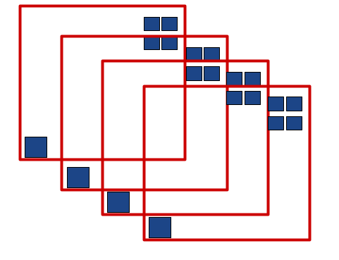
While this particular case gives 4 tiles when only 2 are necessary, this example can be extended with a bit of work to cases where the greedy solution produces arbitrarily bad results. Which inspires deeper examination, despite the solid results on the synthetic benchmark.

Now, the problem here seems to be that we are being too greedy. We are picking up the wrong tiles by trying to include the most tiles. This may work, and yield decent approximations when done globally, but mixed with our left-to-right strategy it doesn’t work as well.

Instead, perhaps, we can be greedy by picking up the tile in the region, furthest to the left. I.e.

1. Take the left-most box in the entire scene (with arbitrary tie-breaks)
2. Take the left-inspection region defined above, and go through the boxes inside that region left to right, fitting in boxes when possible, and shrinking the possible region as necessary to make sure all added boxes will continue to fit inside any tile within the region.

This yields the algorithm that was spoiled at in the top of the post:

Unlike the left-to-right plus greedy case, this algorithm has the beginnings of a worst case analysis that suggests it is a 2-approximation.

1. Consider all the locally left-most boxes. That is, every box that cannot be included in the left-inspection region of some other box.
2. Now, consider that the optimal solution has at least one rectangle for each of these locally left-most boxes. Consider each of these boxes.
3. Now, consider the left-preferring greedy solution applied to all these left-most boxes. After all the boxes in all those greedy tiles are removed, there will be a new set of left-most boxes that appeared from within the left-intersection region of the original set. Now apply the greedy solution to that 2nd set.
4. I claim that step 3 has removed all of the boxes that the optimal set in step 2 removed. (Unfortunately, I don’t have a great argument here, so you are free to try to come up with counter-examples)
5. The resulting set of boxes from step 3 is strictly a subset of step 2. Since the optimal solution cannot increase by removing boxes, you can apply this analysis recursively on the remaining set of boxes.
6. Since step 3 only required at worst twice as many tiles as step 2, this algorithm is a 2-approximation.

To be clear, I’m not super happy about the formal rigor of that argument either. But I can’t come up with any worst case solution worst than a 2-approximation. And my synthetic benchmark labeled it as the best solution yet.

The worst case I could construct is this:

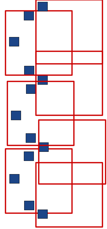
This particular case produces 6 tiles, where the optimal solution produces 4. However, in the infinite limit, extended downwards, this produces twice as many tiles as the best case. Suggesting that the 2-approximation is tight.

Conclusion

The resulting algorithm is better in the worst case and in synthetic benchmarks than both the global greedy algorithm and the left-greedy algorithm. It can be implemented in O(N*log(N)) with a fast data structure, or without any fancy data structure in O(N*sqrt(N)).

And all it required was a bit of care and a bit of persistence!