A Sequential Learning notation for Deep Nueral Archctectures
A Sequential Learning notation for Deep Nueral Archctectures
Most publications and explanations of deep learning have two sorts of explanation types:
- Math that looks like this :
- Diagrams that look like this:
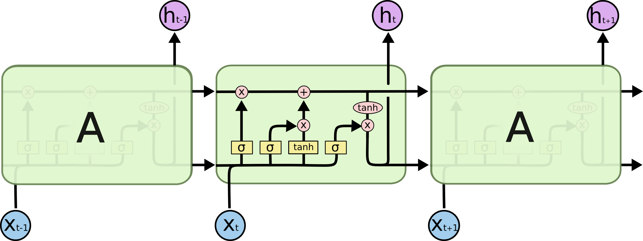
While I must give all credit to Colah’s blog for putting together that excelent diagram, I think it is telling why it is so well known: every other LSTM diagram before that was kind of terrible. Making high quality diagrams is hard, and takes a lot of time and effort.
And it is hard to do math in diagrams—explaining each step will take a lot of time and effort, as each transformation will require a new diagram. So proof-oriented diagrams (like my own here: are extremely time consuming, so you more often see proof written like this:
TERRIBLE LOOKING PROOF HERE
What I am looking for is a notation system that is
- Formal enough to write proofs in
- Expressive enough to write most deep learning archtectures in
- Easily written on a chalkboard, preferably possible to write on a keyboard
I’ll start by example:
Multi Layer Perceptron
To train on observations X and known values y on a 2 layer network via a MSE error
X --[M_1|relu]-> h_1 --[M_2]-> p => y
To train on discrete labels y with a softmax cross entropy error (a bit suprising, but yes, the math checks out)
X --[M_1|relu]-> h_1 --[M_2|softmax]-> p => one_hot(y)
RNN
To train on observation sequence X_t and label sequence y_t using MSE loss,
0 -> h_0
X_t|h_{t-1} --[Enc]-> h_t --[Gen]-> p => y_t
Of course, different functions can be specified for Enc and Gen:
Naive Feed Forward
0 -> h_0
X_t|h_{t-1} --[M_1]-> h_t --[M_2]-> p => y_t
Here Enc can be defined:
GRU
A somewhat computational definition:
0 -> h_0
h_{t-1}|x_t -> c_t
c_t --[R|sigmoid]-> r_t
c_t --[Z|sigmoid]-> z_t
x_t|(h_{t-1}*r_t) --[H|tanh]-> l_t
h_{t-1} * (1 - z_t) + l_t -> h_t
We can define a new macro instead, which will be useful if we want a layered GRU.
Enc: h_{t-1},x_t
    h_{t-1}|x_t -> c_t
    c_t --[R|sigmoid]-> r_t
    c_t --[Z|sigmoid]-> z_t
    x_t|(h_{t-1}*r_t) --[H|tanh]-> l_t
    h_{t-1} * (1 - z_t) + l_t -> h_t
    return h_t
h_0 := 0
h_{t-1},x_t --[Enc]-> h_t
LSTM
0 -> c_0
0 -> h_0
h_{t-1}|x_t -> p_t
p_t --[F|sigmoid]-> f_t
p_t --[I|sigmoid]-> i_t
p_t --[C|tanh]-> l_t
o_t --[O|sigmoid]-> o_t
c_{t-1}*f_t + i_t*l_t -> c_t
tanh(c_t)*o_t -> h_t
Deep RL
To define an environment, we need a few custom functions:
reset() -> S_0step(S_{t-1}) -> S_t,O_t,r_t,d_t
(in general, of course, these will not be differentiable)
Basic TD learning
0.999 -> gamma
reset() -> S_0
S_{t-1},a_{t-1} --[step]-> S_t,O_t,r_t,d_t
O_t --[Value]-> V_t => V_{t-1} * gamma + r_t
A2C with sepearate value and policy networks and
0.999 -> gamma
reset() -> S_0
S_{t-1} --[step]-> S_t,O_t,r_t,d_t
O_t --[Value]-> V_t => V_{t-1} * gamma + r_t
V_{t+1}*gamma + r_t - V_t -> A_t
O_t --[clip_grad(Policy)]-> pi_t $ A_t * log(pi_t)
A2C with generalized advantage
This one is interesting because there is forward looking logic: very hard to implement in a general and efficient way (likely there would have to be some point where gamma^nlam^n is rounded to 0 and ignored…. However, it is fairly easy to write down.
0.999 -> gamma
0.95 -> lam
reset() -> S_0
S_{t-1} --[step]-> S_t,O_t,r_t,d_t
O_t --[Value]-> V_t => V_{t-1} * gamma + r_t
V_{t+1}*gamma + r_t - V_t -> TD_t
TD_t + gamma * lam * A_{t+1} * (1-d_t) -> A_t
O_t --[clip_grad(Policy)]-> pi_t $ A_t * log(pi_t)
TD Learning with GRU
Taking the Enc definition from the GRU implementation:
0.999 -> gamma
reset() -> S_0
S_{t-1} --[step]-> S_t,O_t,r_t,d_t
0 -> h_0
O_t,h_{t-1} --[Enc]-> h_t
h_t --[Value]-> V_t => V_{t-1} * gamma + r_t
DQN
DQN requires a buffer, which is a bit of a weird sort of function/parameter combo
Specialized buffer functions include:
- Add_B(O, a, O’, d) -> none
- Get_B() -> O, a, O’, d
There is also a small complexity of adding an action sampling method….
0.999 -> gamma
reset() -> S_0
S_{t-1} --[step]-> S_t,O_t,r_t,d_t
O_{t-1} --[Q]-> q_{t-1} $ r_t + one_hot(argmax(q_t))
Low level syntax
Three primitive concepts:
- states
- parameters
- functions
- transforms
States
States are local variable definitions. States are immutable and local to a single input value(possibly shared across time). State definitions have attributes
- Name
- Context (usually time)
A reference to a state is accesed with the notation: <Name>_<context> (with the context being optional, by default given context 0.
Parameters
Parameters are global variable definitions that are shared across all data points and all contexts. Parameter instantiations are mutable, and by definition, they have the following attributes:
- Name
- Shape (will be assigned a default shape, some langauge features will be avaliable without the shape being fully defined.
Functions
Functions operate on states and update parameters.
3 rules define a function:
- Forward: (In, Params) -> Out
- Autodiff: (In, Out, Params) -> ^In
- Update: (In, Out, Params) -> ^Params
If f is a stateless function (like relu) then Update() will accept and return an empty set of parameters. If f is a non-differentiable function (like one-hot) then Autodiff will additionally return constant zeros for its inputs.
Builtin functions include:
dense_M(x)conv_K(x)add(x,y)exp(x)batch_norm(x)dropout(x)
Transforms
Transforms operate on functions (essentially higher order functions). Transforms have 3 major operations
- ForwardTransform: (InForwards,) -> OutForward
- AutodiffTransform: (Autodiffs,) -> Autodiff
- UpdateTransform: (Updates,) -> Update
Some special transform include:
- compose (Chains outputs of function a to inputs of function b, composes updates and autodiff)
- nograd (makes AutoDiff return 0s)
- adam_opt (Adds new parameters, changes UpdateTransform via adam rule)
Syntax transformation rules
Implementation
Implementation should be able to generate any low level tensor code, for example: pytorch code.
Syntax transformations
AST manipulations, transformation rules, and static optimization proceedures should occur in a proper functional language, such as OCaml.
C extension functions
Features like RL environments and replay buffers should use C extensions to execute the functions. Proper support for these may include required type definitions and code generation.
Decent library support to wrap these into functions is required.
Proposed batch implementation
- Each state has a batch dimention.
- This batch dimention can take on any power of 2.
- Data will alway be contiguous in the batch dimention.
- Each seperate state computation can have a different batch size.
- If a dependent function requests a larger batch size, then it can wait until the function is executed multiple times, and the data placed in contiguous memory.
- If a dependent function requests a smaller batch size, it can execute multiple times before waiting on the data to be generated
Context/time implementation
- A backwards and forwards horizon should be specified to handle edge cases in implementation.
- Conceptually, this should generate an infinite sequence of variables, and rely on garbage collection to free up memory.
- Practically, this should only roll out for horizon steps.
Caching vs Recomputation
There are performance/memory tradeoffs which occur when doing recurrent or RL methods on whether caching or recomputation is best.
The static optimizer should try some combinations and determine what is the best tradeoff.